VLA Low-band Ionosphere and Transient Experiment (VLITE)
Ionosphere
Ionospheric Analysis
The ionosphere analysis portion of VLITE is dedicated to the study of fine-scale (~1-10 km)
ionosphere dynamics and the relationship to larger structures (hundreds of km). The VLA
low-band systems have virtually unmatched sensitivity to fluctuations in the ionosphere
total electron content (TEC), the integrated density of free electrons along a line of
sight. When observing a bright cosmic source, these systems can be used to characterize TEC
fluctuations more than two orders of magnitude weaker than those detectable with similar
GPS-based methods. Such fluctuations are prevalent on smaller scales, making the VLA an
excellent instrument for probing fine-scale ionosphere dynamics. Many continuously operating
GPS receivers within New Mexico are also being used to simultaneously study larger-scale
fluctuations. The (nearly) continuous data stream delivered by VLITE, when combined with
this GPS data, constitutes a singular data set for the study of coupling mechanisms among
fine-, medium-, and large-scale ionosphere dynamics. In addition, such a continuous flow of
data allows for the characterization of the fine-scale ionosphere response to relatively
rare space weather, atmospheric, and/or seismic events such as solar flares
(Helmboldt et al. 2015), large storms,
earthquakes, and explosions (Huang et al.
2019) that would be missed by proposal-based, low-band observing.
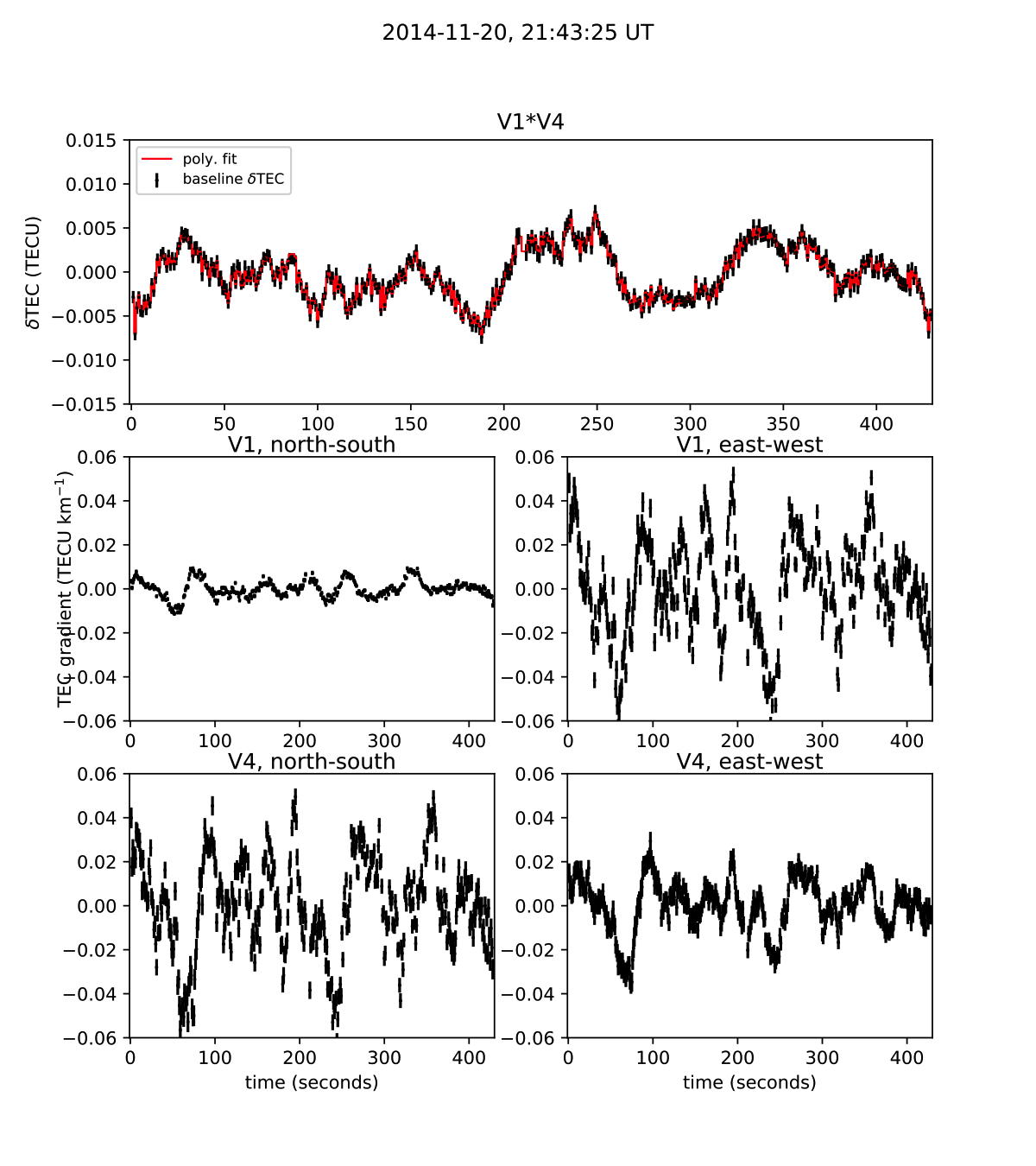
Example of antenna-based TEC gradients from November 11, 2014 observation of the Galaxy
cluster Abell 2052 (A2052). The upper panel shows the δTEC time series for the
V1*V4 antenna baseline (black points) with the values from a polynomial fit to all
baselines used to determine the TEC gradients (red). The north-south and east-west
components of the gradient are shown in the remaining panels for antennas V1 and V4.
Reproduced from Helmboldt et al. 2019).
The ionosphere pipeline is optimized to sense fluctuations on small temporal (~seconds),
spatial (~few km), and amplitude (~10-3-10-4 TECU km-1)
scales. Because the δTEC values represent antenna-based effects that dominate on
short time scales (~minutes or less), the general approach to signal processing is as
follows:
Extract good visibility phases from the raw data, while flagging obviously aberrant data.
Unwrap the phase time series and de-trend to remove slowly varying instrumental and/or source contributions.
Determine and remove contributions from baseline-based errors.
Use final δTEC time series to compute TEC gradients.
Please see Helmboldt et al. 2019
for more details on VLITE and its ionospheric pipeline.
Plasmaspheric Analysis
Between the ionosphere and the solar wind-driven outer magnetosphere is a region of
relatively cold, co-rotating plasma known as the plasmasphere. Magnetic field-aligned
irregularities with longitudinal scales of tens of km were discovered with the VLA low-band
system in the early 1990s
( Jacobson & Erickson 1992).
These were first identified as relatively fast moving/oscillating waves directed toward
magnetic east until it was realized that the high speed was due to co-rotation at a
relatively large distance (thousands of km). Using archival VLA low-band data and VLITE
data, a method was recently developed to produce range/time-resolved images of these
structures, sometimes called co-rotating plasmaspheric irregularities (CPIs;
Helmboldt et al. 2020). This method
spectrally decomposes the time series of TEC gradients measured using the methods described
above into several frequency bands. A phase velocity is then estimated for each of the
higher-frequency oscillation bands most likely to be CPIs. Because their motions are
dominated by co-rotation, the magnitude of this velocity gives the distance to the
disturbance. A check is made to confirm that the velocity direction is consistent with what
is expected for a CPI. Following this, the data from all bands are recombined to form a
range/time image (see an example below). A separate pipeline runs daily to identify any
observations of bright calibrators longer than five minutes in duration and performs this
imaging analysis on those data.
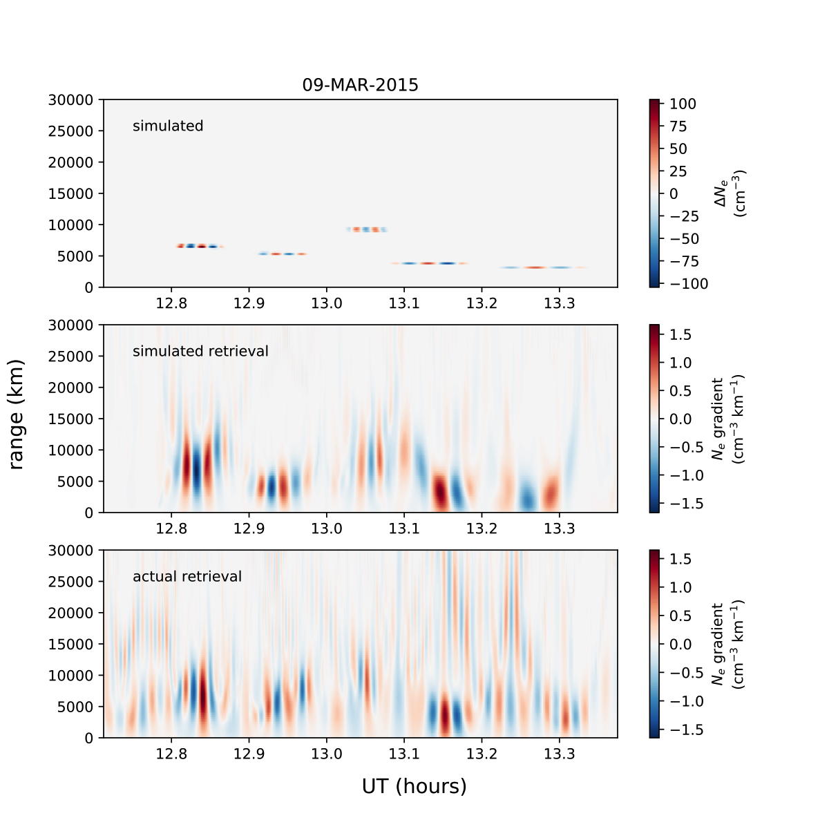
Derived from VLITE observations of a bright calibration source, range/time-resolved
images of CPIs (lower panel). The upper panel shows the change in electron density
within the plasmasphere as a function of range and time due to a series of planewave
electric field disturbances patterned after previous observations of such phenomena with
coherent backscatter radars. The middle panel shows a simulated retrieval using the CPI
imaging methods describe above, which is qualitatively similar to the actual
observations. Reproduced from
Helmboldt et al. 2020.